Prerequisites
- You are using dbt to orchestrate your BigQuery workloads.
- Your GCP billing export is connected to Costory.
Output
- Cost visibility broken down by dbt model, team, package, or any custom label.
- Ability to identify which models drive auto-scaling or high processing costs.
- Foundation for cost allocation and optimization.
Steps
Label your dbt operations in BigQuery
Configure automated labels in your Then create a macro
This macro will label every query run during the dbt run.
dbt_project.yml so every query is tagged with dbt native metadata:bq_labels to populate the labels automatically. Here is all the information you can use:| Object | Property | Description |
|---|---|---|
| Node | node.original_file_path | The original file path of the node |
| Node | node.name | The name of the node |
| Node | node.resource_type | The resource type of the node (model, test, seed, snapshot, table) |
| Node | node.package_name | The dbt package name |
| Node | node.database | For BigQuery, this is the project name of the project on which you write |
| Node | node.schema | The dbt schema of the node |
| env_var macro | ex: env_var(‘username’,‘cloud_run_task’) | Any env var available at runtime |
| var macro | ex: var(‘customer’, ‘test’) | Any dbt variable available at runtime |
| target | target.get(‘profile_name’) | The profile name of the target (useful if you split per target your ingested / full refresh / backfill jobs) |
| target | target.get(‘target_name’) | The target name of the target |
Label your storage resources
In BigQuery, storage costs are visible at the dataset level using You can also set labels at the
resource_id / resource_name, but they are not visible at the billing level per table. To add labels at the table level, apply them in your dbt model config:dbt_project.yml level. Note that project-level labels will override model-level labels if both are set.Visualize your labeled job costs without Costory
Use BigQuery’s To query storage-level labels on tables:
INFORMATION_SCHEMA to analyze costs by label:Visualize your labeled job costs with Costory
-
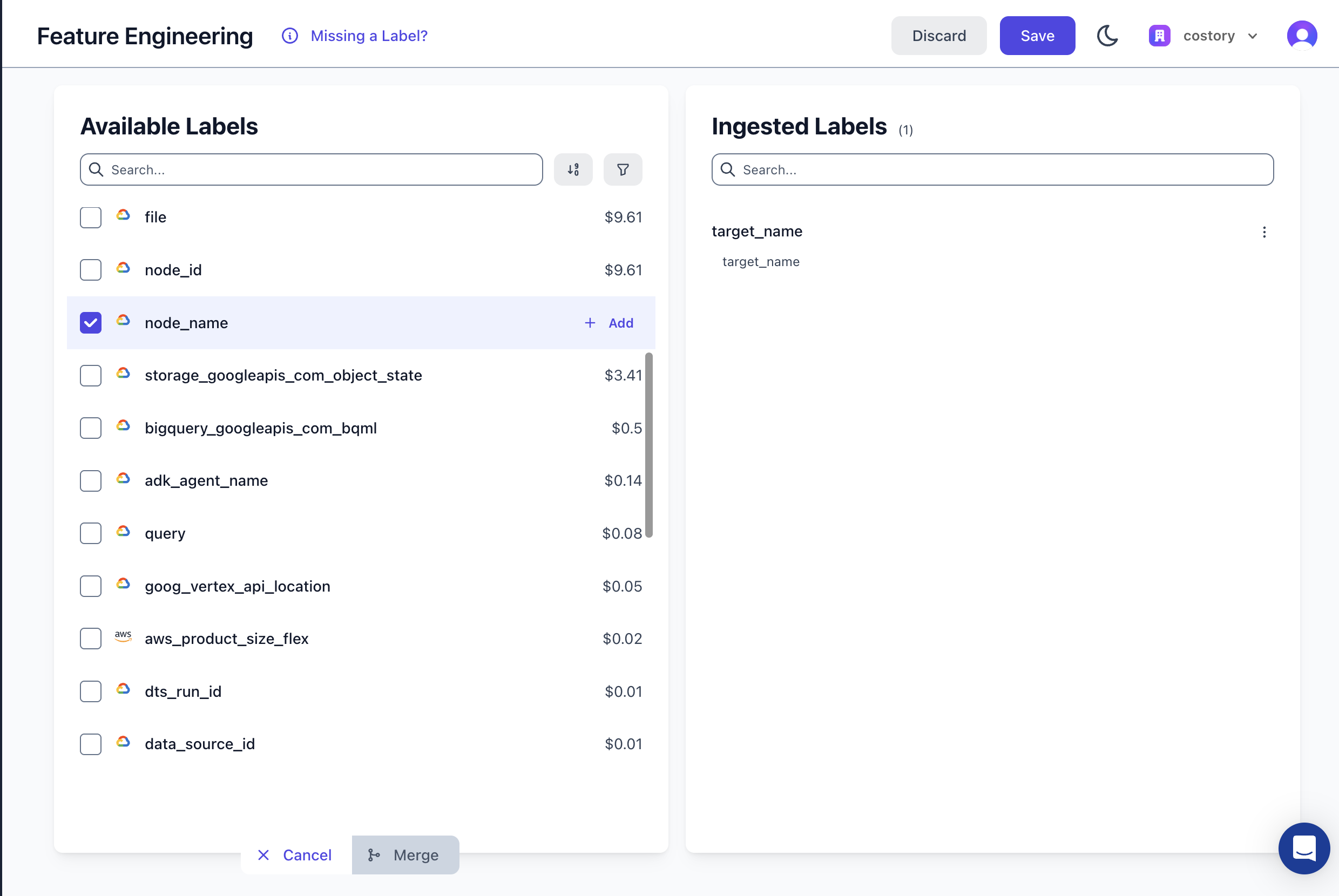
Ingest the labels into Costory using the feature engineering UI:
-
If part of your BigQuery labels should be merged within an existing label, use the merge feature to combine two labels into one (e.g.,
k8s_label_appandapp). -
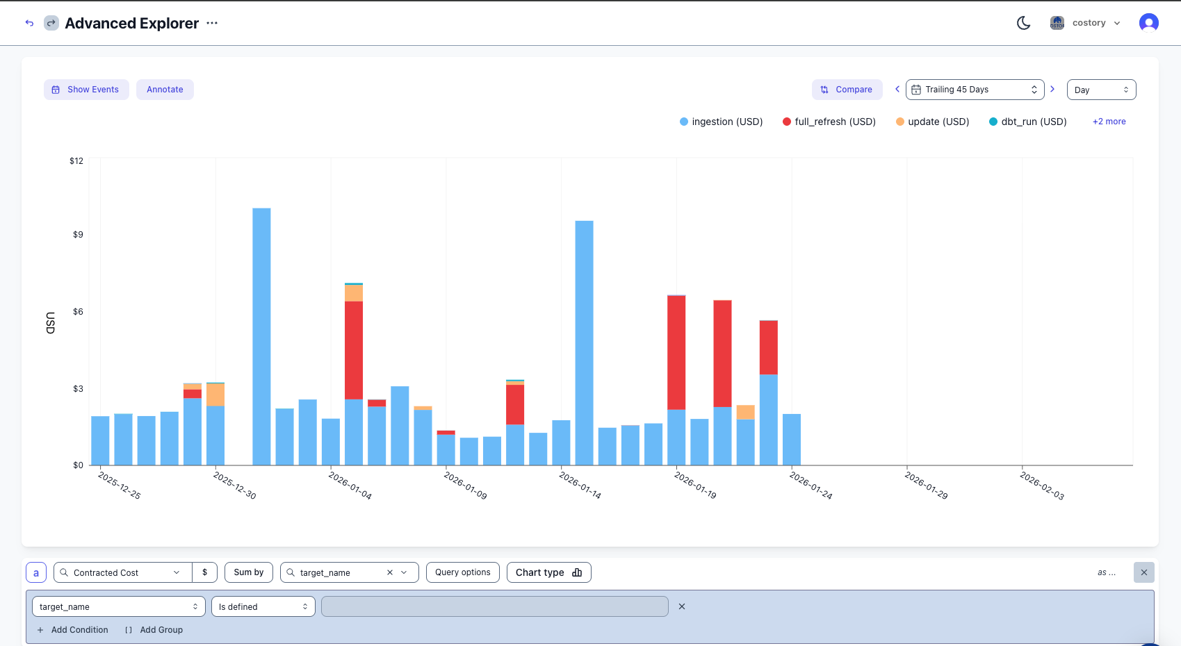
Create a virtual dimension to allocate the cost, or explore costs directly in Explorer:
Best practices
Labels
- Ingest
node_namefor fine-grained cost investigation to understand which exact model is driving cost. - Use
package_nameorschemato map each schema to the correct team or owner. You can formalize this mapping with virtual dimensions. - Use
target_nameto split daily jobs, full refreshes, and backfills.
Quotas
- Set a quota on GCP for query bytes billed per service account or per user using
QueryUsagePerUserPerDay.
Alerts
- Set an alert close to the daily average on ingestion costs. Daily ingestion jobs should be very stable.
- For full refresh jobs, evaluate alerts over a larger period to avoid false positives from spikes.
Storage costs
- Evaluate storage costs frequently. After 90 days the storage price decreases, but if you never read the data you should rely on an expiration policy instead.
- Since 2023, you can choose per dataset the storage billing model:
- Logical storage: you pay based on the logical size (before compression).
- Physical storage: you pay based on the physical size (after compression).
region-us suffix:
Next steps
- Explore your costs in Explorer: slice and dice your BigQuery spend with full context.
- Tag & allocate costs with dimensions: map labels to teams and build cost allocation rules.
- Allocate shared Cloud SQL costs across teams: apply similar labeling strategies to Cloud SQL.
- Get Kubernetes cost visibility with EKS: extend cost tracking to your container workloads.
FAQ
What BigQuery labels does dbt support?
What BigQuery labels does dbt support?
dbt supports job-level labels via
query-comment in dbt_project.yml and table-level labels via the labels property in model config(). Job labels appear in INFORMATION_SCHEMA.JOBS_BY_PROJECT, while table labels appear in INFORMATION_SCHEMA.TABLE_OPTIONS.What's the difference between physical and logical storage costs?
What's the difference between physical and logical storage costs?
Physical storage costs are the costs of the data stored in BigQuery. Logical storage costs are the costs of the data stored in BigQuery after compression. You can compare both costs using the SQL query above.
Usually tabular data with frequent values compresses well, so the physical cost is typically lower than the logical cost.
How do I set a BigQuery cost quota?
How do I set a BigQuery cost quota?
Use GCP’s custom quotas feature with
QueryUsagePerUserPerDay to limit bytes billed per user or service account per day.Will project-level labels override model-level labels?
Will project-level labels override model-level labels?
Yes. Labels set in
dbt_project.yml at the project level will override labels set in individual model config() blocks if both define the same key.Can I track BigQuery costs per query when using Slots?
Can I track BigQuery costs per query when using Slots?
When using slots, you will need to reattribute the slots costs to each query. You can do this using virtual dimensions. A native connector is under development to do it natively.